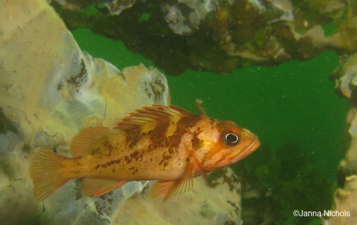
Rockfish (genus Sebastes) are an important commercial and recreational fishing target on the west coast. The early life stages of Rockfish are spent in the water column until they grow strong enough to swim to structure. With global ocean temperatures increasing, I aim to analyze how increases in water temperature during Pelagic Larval Duration (PLD) affects the abundance of new rockfish, or Young of Year (YOY). I will utilize timeseries data of YOY abundance collected at the Northern Channel Islands. During data collection, California experienced a marine heatwave often referred to as “The Blob” during 2014-2016. I will analyze the effects of temperature on YOY abundance from 2012 to 2019 in order to determine if the warmer waters during the Blob influenced abundance and give insight to how the population may change has global ocean temperatures increase due to climate change. Additionally, I will incorporate the impacts of upwelling, which supplies nutrients to YOY during the PLD.
About the data
The data quantifying Rockfish recruitment comes from the Partnership of Interdisciplinary Sciences of Coastal Oceans (PISCO) long-term fish recruitment monitoring in the Channel Islands. The YOYs were collected using Standardized Monitoring Units for the Recruitment of Fishes (SMURFs) that were placed just off the coast of the Northern Channel Islands in an attempt to collect recruit fish as they swam to structure. Monitoring took place from 2000-2018, with collections occuring year round starting in 2012.
NOAA data is used to quantify temperature with Sea Surface Temperature (SST) lag 30 days from time of collection to predict SST during PLD. Upwelling was quanitified using the Biological Effective Upwelling Transport Index (BEUTI) lag 30 days.
Hypotheses
H0: Temperature has no effect on rockfish recruitment
Ha: Increased temperature has an effect on rockfish recruitment
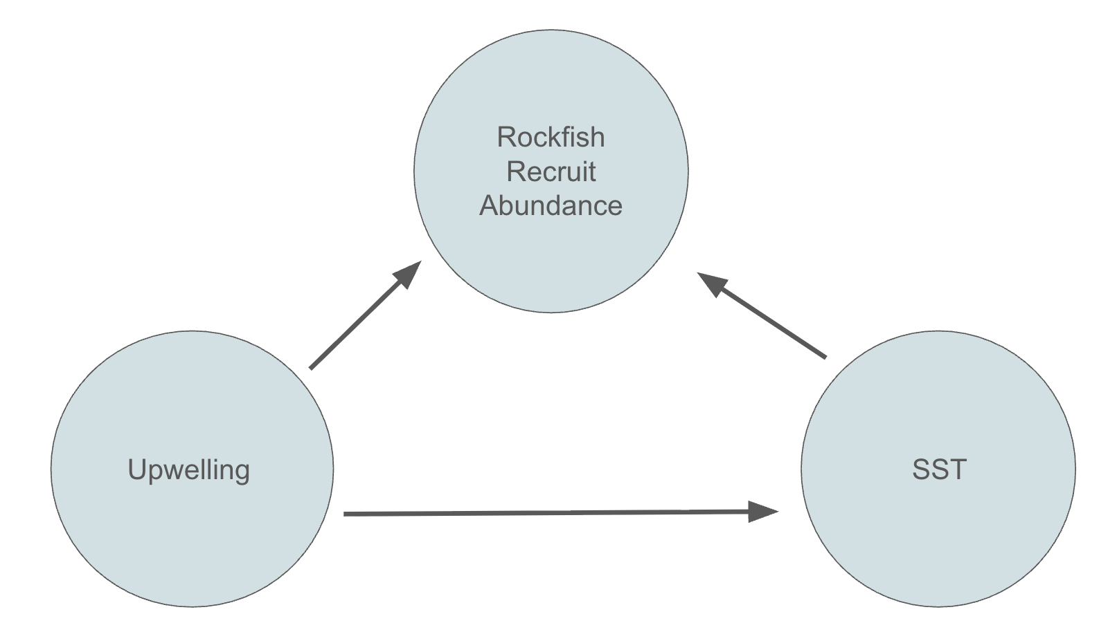
Directed Acyclic Graph (DAG)
Upwelling is the result of moving water, often bringing cold, nutrient rich water from the deep up to the surface. This impacts the SST, decreasing temperature during mass upwelling events. Additionally, the nutrients supplied in upwelling have a direct impact on YOY development, providing necessary nutrients during the PLD. Temperature also impacts fish development in the PLD, with faster development occurring at warmer temperatures.
Load necessary packages and data
Code
library(tidyverse)library(knitr)library(pscl)library(modelsummary)library(MASS)smurf <-read_csv("data/PISCO_UCSB_subtidal_recruitment_fish_data.1.2.csv")smurf_sp <-read_csv("data/PISCO_UCSB_subtidal_recruitment_fish_spp_list.1.2.csv")# Data for ocean temperature and upwellingocean <-read_csv("data/ALL_OCEAN_DATA.csv")
Data Cleaning
Before I can start working on my statistical modelings, I need to do some cleaning and filtering to get the data ready to be analyzed. I first subset my data to include only my species of interest. I chose Copper, Kelp, Gopher, Grass, and Brown rockfish, because they have similar PLDs and are difficult to differentiate at a small size. I chose to look at data between 2012-2018 to include two years before and after the Blob. I also narrowed the window of sampling by year to only include sampling during the months of recruitment to avoid a seasonal pattern from emerging. I chose to only look at the two most consistently sampled sites, which were located at Santa Cruz island.
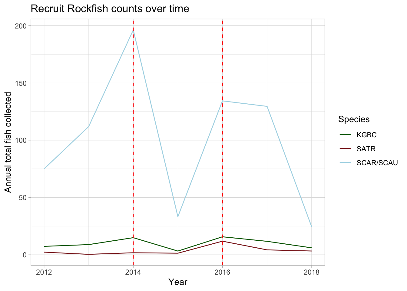
ggplot(rf_yoy_av, aes(year, av_fish)) +geom_line(aes(color = classcode)) +geom_vline(xintercept =2014, color ="red", linetype ="dashed") +geom_vline(xintercept =2016, color ="red", linetype ="dashed") +scale_color_manual(values =c("darkgreen", "brown4", "lightblue")) +labs(x ="Year",y ="Annual total fish collected",title ="Recruit Rockfish counts over time",color ="Species") +theme_light()
The red-dashed lines denote the beginning and end of the blob. Rockfish YOY abundance began increasing in the years leading up to the blob while the waters gradually warmed. Naturally the abundance dipped after reaching a peak, but began to climb again during the marine heat wave, suggesting that the warmer waters could have been beneficial for YOY development.
In order to analyze this data, I selected a hurdle model because the data contains many 0’s. Hurdle models are a type of hierarchical model that first test presence and absence (0 and 1), then tests abundance without 0’s. The presence-absence model is written using a Binomial regression: \[FishPresence \sim Binomial(1, p) \]
For simplicity in understanding the model, I only selected temperature as predictor variable to simulate data and return my selected beta values. To begin simulating data, I need to generate x values representing the temperature data. From there, I can use those temperatures and beta values I selected to run the binomial equation to find logit(p). I then can take the inverse logit of those values to generate p which represents the probability of success. Using that probability, I simulated a success variable with rbinom() to generate 0’s and 1’s.
Similar to the binomial step, I chose new beta values for the equation and used the same generated temperature data. The output of the negative binomial equation gives log of mu, or the mean. By applying an exponential to that, the mean of the predicted data is found, which is then used to simulate count data using rnbinom(). Actual abundance can be calculated by multiplying the simulated success and abundance together.
I can create a prediction grid by generating SSTs from my real data ranges and keeping the upwelling index constant by taking the mean. While the upwelling index often seasonally fluctuates in the real world, I will assume a constant value because I am only looking at recruitment during a short period during the year. Keeping it constant will create simplicity while interpreting the model predictions. I will use bootstrapping to resample the original data set with replacement and apply the hurdle model to make predictions for the mean YOY abundance.
Code
pred_grid <-expand_grid(SST_D30 =seq(min(rf_yoy$SST_D30, na.rm =TRUE),max(rf_yoy$SST_D30, na.rm =TRUE),length.out =1000),beuti_30 =mean(rf_yoy$beuti_30))# reiterate through the boot 1000 timesboot <-map_dfr(1:1000, \(i) {# sample with replacement boot_sample <-slice_sample(rf_yoy, n=432, replace =TRUE)# run a beta regression on every single boot sample boot_mod <-hurdle(total_fish_collected ~ SST_D30 * beuti_30, data = boot_sample,dist ="negbin",zero.dist ="binomial")# predict the boots values (the outcomes are best fit lines)mutate(pred_grid,count =predict(object = boot_mod,newdata = pred_grid,type ="response"),boot = i)})
I also can predict the mean YOY abundance using the entire population to create a best fit line for the model.
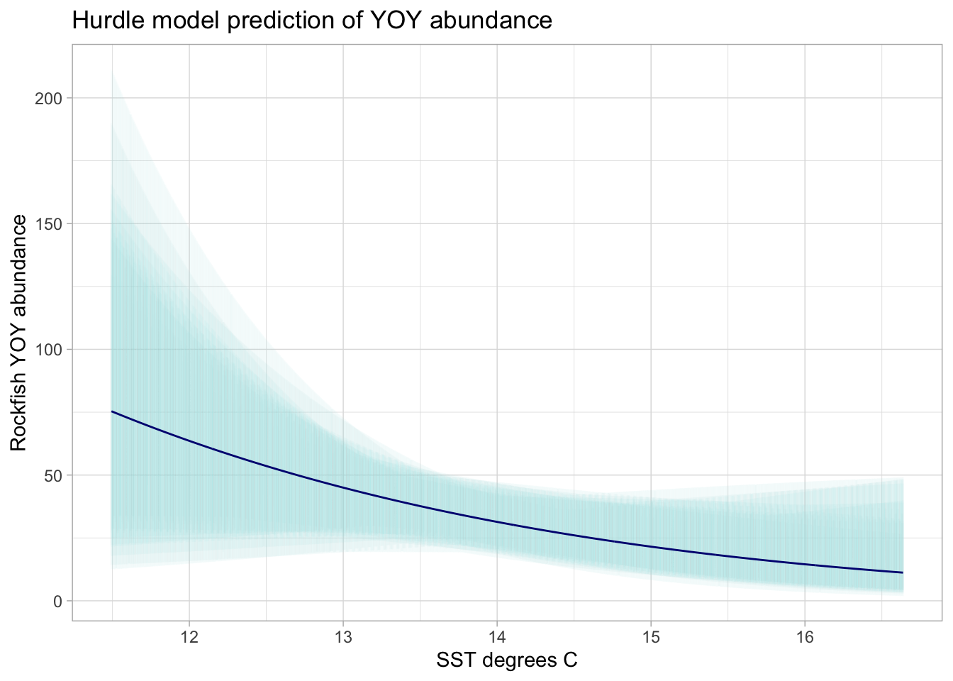
ggplot(boot, aes(SST_D30, count)) +geom_line(color ="lightblue", alpha =0.05) +geom_line(data = pred_hurdle_model, aes(SST_D30, count), color ="navy") +labs(x ="SST degrees C",y ="Rockfish YOY abundance",title ="Hurdle model prediction of YOY abundance") +theme_light()
The confidence intervals are visualized through the bootstrapped values. According to the predictions, at an SST of 11.5 degrees C, we are 95% confident the mean YOY abundance would fall between 25 and 175. On the higher end of the temperature range, around 16.5 degrees C, we are 95% confident the mean abundance of YOY’s would fall between 0 and 60. The narrowest CI occurs around 14 degrees C, where we are 95% confident the mean value falls between 20 and 45 YOY. Additionally, there appears to be a negative relationship between SST and rockfish YOY abundance. Without further statistical testing, I cannot conclude from the data whether temperature had an effect on rockfish recruitment, leading me to fail to reject my null hypothesis. However, further testing is required to come to a conclusion on the effects of temperature on rockfish recruitment.
BONUS! Hurdle model without upwelling predictor variable
To determine the influence of the upwelling index on the model, I can rerun the previous bootstrapping and true population model fit to observe how only temperature influences YOY abundance predictions.
Code
pred_grid2 <-expand_grid(SST_D30 =seq(min(rf_yoy$SST_D30, na.rm =TRUE),max(rf_yoy$SST_D30, na.rm =TRUE),length.out =1000))# reiterate through the boot 1000 timesboot2 <-map_dfr(1:1000, \(i) {# sample with replacement boot_sample <-slice_sample(rf_yoy, n=432, replace =TRUE)# run a beta regression on every single boot sample boot_mod <-hurdle(total_fish_collected ~ SST_D30, data = boot_sample,dist ="negbin",zero.dist ="binomial")# predict the boots values (the outcomes are best fit lines)mutate(pred_grid2,count =predict(object = boot_mod,newdata = pred_grid2,type ="response"),boot = i)})
Code
true_hurdle_model2 <-hurdle(total_fish_collected ~ SST_D30, data = rf_yoy,dist ="negbin",zero.dist ="binomial")
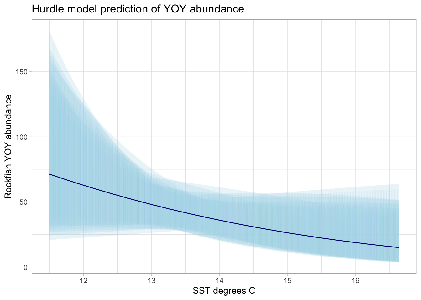
ggplot(boot2, aes(SST_D30, count)) +geom_line(color ="lightblue", alpha =0.1) +geom_line(data = pred_hurdle_model2, aes(SST_D30, count), color ="navy") +labs(x ="SST degrees C",y ="Rockfish YOY abundance",title ="Hurdle model prediction of YOY abundance") +theme_light()
Without upwelling, temperature appears to have less of an effect on YOY abundance. Additionally, the CI at both tail ends are noticebly larger than in the model that includes upwelling. While no definitive conclusions can be made from the data visualization about the impacts of SST and upwelling, there does appear to be a negative relationship between temperature and YOY abundance, with that relationship strengthening with the addition of upwelling.
References
ERDDAP - SST, Aqua MODIS, NPP, 0.0125°, West US, Day time (11 microns), 2002-present (1 Day Composite) - Data Access Form. (2016). Noaa.gov. https://coastwatch.pfeg.noaa.gov/erddap/griddap/erdMWsstd1day.html
Jennifer E. Caselle, Peter M. Carlson, Chris Honeyman, Avrey Parsons-Field, & Katie D. Koehn. (2020). PISCO UCSB Subtidal Fish Recruitment Data. PISCO MN. doi:10.6085/AA/PISCO_UCSB_Fish_Recruitment.1.3.
 Upwelling is the result of moving water, often bringing cold, nutrient rich water from the deep up to the surface. This impacts the SST, decreasing temperature during mass upwelling events. Additionally, the nutrients supplied in upwelling have a direct impact on YOY development, providing necessary nutrients during the PLD. Temperature also impacts fish development in the PLD, with faster development occurring at warmer temperatures.