Visualizing fire scars from the 2025 Eaton and Palisades fires

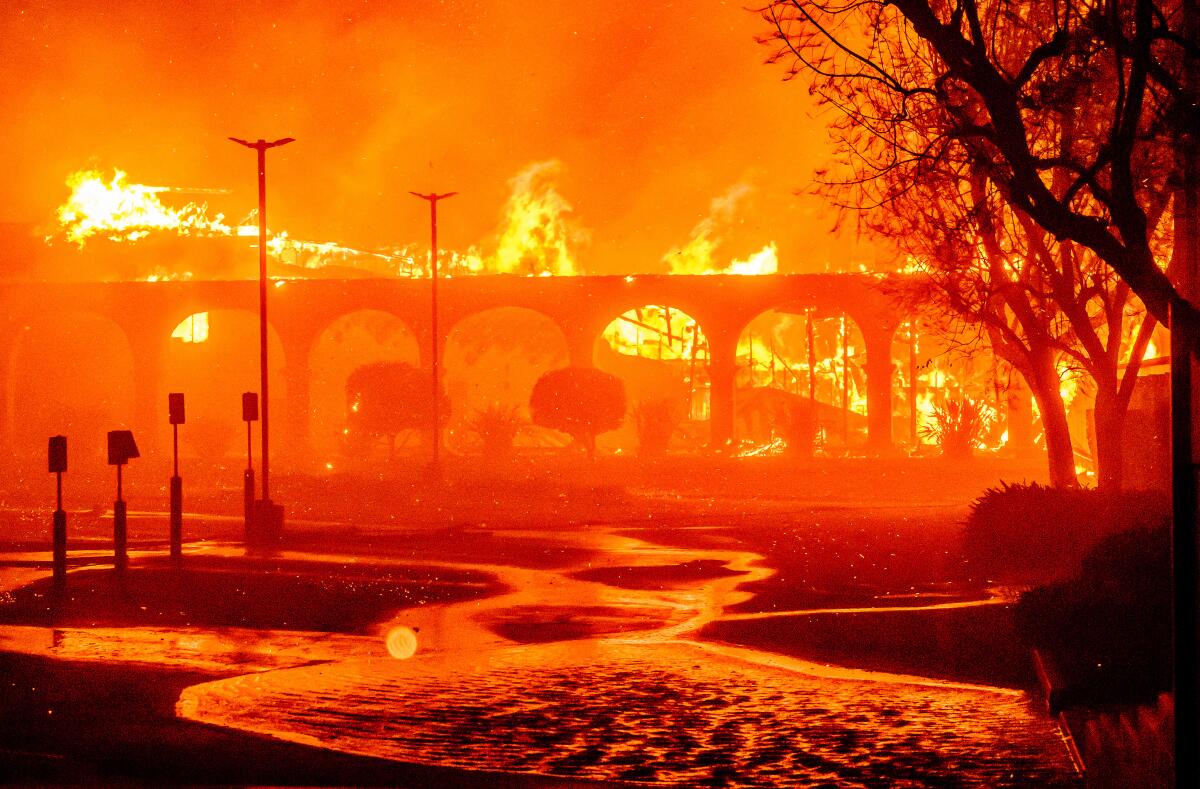
More information for this project can be found on the GitHub Repository

About

In 2025, the Los Angeles area experienced two massive fires perpetuated by stong Santa Ana winds and dry brush. Though on opposite sides of the county, the Eaton and Palisades fires burned almost in unison and primarily impacted Altadena near Pasadena and Palisades near Malibu. As a result, over 16,000 homes and businesses were destroyed and 31 lives were lost (stat from Los Angeles County). The fires lasted 24 days, however both communities are still rebuilding after the tragedy. This project visualizes the aftermath and burn scars of the Palisades and Eaton fires with satellite images and geospatial data.

Highlights:

Work with and visualize raster data using xarray and NetCDF datasets
Analyze false color images with satellite imagery by using different reflectance wavelengths
Visualize raster and geographic data together to determine areas with fire scars
Examine socioeconomic demographics of areas affected by the fires

Data

This notebook contains datasets with the perimeters of the Palisades and Eaton fires and reflectance satellite imagery of the Los Angeles area following the fires. The perimeter data comes from the ArcGIS hub and can be downloaded here. The other dataset is a NetDCF comes from the Microsof Planetary Computer data catalogue and was collected by the Earth Resources Observation and Science (EROS) Center and can be downloaded from this shared Google Drive.

Socioeconomic data was quatified by the Environmental Justice Index data from Centers for Disease Control and Prevention and Agency for Toxic Substances Disease Registry.

References:

Centers for Disease Control and Prevention and Agency for Toxic Substances Disease Registry. [2025] Environmental Justice Index. Accessed [Dec. 3, 2025]. https://atsdr.cdc.gov/place-health/php/eji/eji-data-download.html

Earth Resources Observation and Science (EROS) Center. (2020). Landsat 8–9 Operational Land Imager / Thermal Infrared Sensor Level-2, Collection 2 [Dataset]. U.S. Geological Survey. https://doi.org/10.5066/P9OGBGM6 [Accessed Nov. 22 2025]

Los Angeles County Enterprise GIS. (2025). Palisades and Eaton Dissolved Fire Perimeters [Dataset]. Los Angeles County. https://egis-lacounty.hub.arcgis.com/maps/ad51845ea5fb4eb483bc2a7c38b2370c/about [Accessed Nov. 22 2025]

Import necessary packages

We start by importing geopandas and xarray which are necessary reading geopsatial data. We will also use matplotlib.pyplot for visualization.

# Import packages
import pandas as pd
import numpy as np
import geopandas as gpd
import os
import xarray as xr
import matplotlib.pyplot as plt

Fire perimeter data and exploration

We use known fire perimeter data for the Palisades and Eaton fires from the ArcGIS hub.

Before we start working with the data, it’s important to understand what the data actually looks like and represents. The fire perimeter data is imported and explored to understand the type of data and approaches for visualization. We will look at the CRS and data types in each column.

# Read in Palisades perimeter data
fp1 = os.path.join('data', 'Palisades_perm_20250121', 'Palisades_Perimeter_20250121.shp')
pal_perm = gpd.read_file(fp1)

# Read in Eaton perimeter data
fp2 = os.path.join('data', 'Eaton_perm_20250121', 'Eaton_Perimeter_20250121.shp')
eat_perm = gpd.read_file(fp2)

# Look at CRS of perimeter datasets
print('Palisades perimeter CRS:', pal_perm.crs)
print('Eaton perimeter CRS:', eat_perm.crs)

Palisades perimeter CRS: EPSG:3857
Eaton perimeter CRS: EPSG:3857

# Look at column types
print('Palisades perimeter dtypes:\n', pal_perm.dtypes)

Palisades perimeter dtypes:
 OBJECTID         int64
type            object
Shape__Are     float64
Shape__Len     float64
geometry      geometry
dtype: object

print('Eaton perimeter dtypes:\n', eat_perm.dtypes)

Eaton perimeter dtypes:
 OBJECTID         int64
type            object
Shape__Are     float64
Shape__Len     float64
geometry      geometry
dtype: object

Through exploration, it was determined that both perimeters have a projection of EPSG:3857. Both datasets are fairly similar, only containing spatial data in both numeric and geometric types.

Landsat data and exploration with NetCDF

To actually visualize the fire scars, we utilized reflectance satellite imagery of the Los Angeles area following the fires. This data comes from Microsof Planetary Computer data catalogue and was collected by the Earth Resources Observation and Science (EROS) Center. This data is multi-dimensional, containing a collection of bands (red, green, blue, near-infrared and shortwave infrared) from the Landsat 8 satellite.

The Landsat data is analyzed using the Network Common Data Form (NetCDF). NetCDF data is imported and explored to determine the ways it can be visualized and paired with the perimeter datasets. We explore the data in a similar way to the perimeter data,

landsat = xr.open_dataset('data/landsat8-2025-02-23-palisades-eaton.nc')
landsat.head()

The landsat dataset is 3-dimensional with x and y geographic dimensions and the third being time. The data has six variables, red, green, blue, nir08, swir22, spatial_ref, 5 of which measure different waves of light reflectance.

Restoring geospatial information

Upon exploration, we determined that the landsat data is not a geospatial object. Using NetCDF with data does not present geospatial in the same way as we would expect from geopandas dataframes. In order to work with both the landsat data and the perimeter data, we need to standarized the geographic projections to visualize the data together. This can be done by accessing the spatial reference variable to determine the projection.

# Use `spatial_ref.crs_wkt` to access spatial reference variable
landsat_crs = landsat.spatial_ref.crs_wkt

# Assign CRS as previously accessed spatial reference variable
landsat = landsat.rio.write_crs(landsat_crs)


print(f'The CRS of the Landsat data is {landsat.rio.crs}')

The CRS of the Landsat data is EPSG:32611

We need to determine if there are any NA’s in any of the band variables.


for band in landsat.data_vars:
    print(band, landsat[band].isnull().any().item())

red False
green True
blue True
nir08 False
swir22 False

landsat = landsat.fillna(0)

False color map with fire perimeters

A false colored image displaying inrafred and near infrared false color images with the fire perimeters is created. In this image there is a clear distinction of vegetation and other land coverage between places that did and did not experience fires.

# Need to fix CRS's of perimeters
pal_perm = pal_perm.to_crs(landsat_crs)
eat_perm = eat_perm.to_crs(landsat_crs)

fig, (ax) = plt.subplots( figsize=(22, 10))

# Plot false color image
landsat[[ "swir22", "nir08", "red"]].to_array().plot.imshow(robust = True, ax=ax)
plt.title('False Color Image of Los Angeles area following the Palisades and Eaton Fires of 2025', size = 20)

# Plot Eaton and Palisades perimeters
eat_perm.plot(ax=ax, edgecolor = "firebrick", linewidth = 2, color = "none")
pal_perm.plot(ax=ax, edgecolor = "firebrick", linewidth = 2, color = "none")

# Make the aesthetically nicer
ax.axis('off')

# Add labels for fires
ax.text(x = 399000, y = 3790000, s = "Eaton Fires", color = "black", fontsize = 10).set_bbox(dict(facecolor='white', edgecolor = 'none'))
ax.text(x = 347000, y = 3774000, s = "Palisades Fires", color = "black", fontsize = 10).set_bbox(dict(facecolor='white', edgecolor = 'none'))

# Add a description of the figure
plt.figtext(s = "This figure shows the false color imaging with Shortwave infared, near-infared, and red wavelength reflectance to demonstrate the differences in vegetation \nacross the Los Angeles area following the Palisades and Eaton fires that occured in January 2025. The fire perimeters are outlined in red and labeled by location.",
            x = 0.5,
            y = 0.05,
            ha = 'center',
            size = 12,
            wrap = True)
    
plt.show()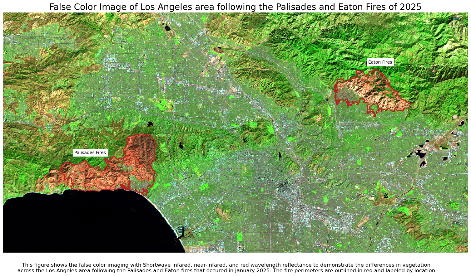

Import and analyze environmental justice data

We use the Environmental Justice Index (EJI) from Centers for Disease Control and Prevention and Agency for Toxic Substances Disease Registry to visualize the socioeconmic demographics within the fire perimeters.

To use the EJI data with the fire perimeter data, the projections must be transformed to combine and visualize the data

fp3 = os.path.join("data", "EJI_2024_United_States", "EJI_2024_United_States.gdb")
eji = gpd.read_file(fp3)

# Update column names to lower case for ease later
eji.columns = eji.columns.str.lower()

# Update CRS's to match EJI data
eat_perm = eat_perm.to_crs(eji.crs)

pal_perm = pal_perm.to_crs(eji.crs)

# Clip EJI data to both fire perimeters
eji_eat = gpd.clip(eji, eat_perm)

eji_pal = gpd.clip(eji, pal_perm)

Create an image of uninsured homes within fire perimeters

We are interested in analyzing socioeconomic demographics of the homes in the fire perimeters. With such extreme damage to many homes in the fires, looking at the amount of uninsured homes using the e_uninsur variable of EJI within the fire perimeters will represent how deterimental these fires were to so many families.

fig, (ax1, ax2) = plt.subplots(1, 2, figsize=(20, 10))

# Select EJI variable of interest: Uninsured homes
eji_variable = 'e_uninsur'

# 
vmin = min(eji_pal[eji_variable].min(), eji_eat[eji_variable].min())
vmax = max(eji_pal[eji_variable].max(), eji_eat[eji_variable].max())

# Census tracts for Palisades fire perimeter
eji_pal.plot(
    column= eji_variable,
    vmin=vmin, vmax=vmax,
    legend=False,
    ax=ax1,
    cmap="PuBuGn"
)
ax1.set_title('Palisades Fire', size = 15) # Give subplot title
ax1.axis('off')

# Pensus tracts for Eaton fire perimeter
eji_eat.plot(end 
    column= eji_variable,
    vmin=vmin, vmax=vmax,
    legend=False,
    ax=ax2,
    cmap="PuBuGn"
)
ax2.set_title('Eaton Fire', size = 15) # Give subplot title
ax2.axis('off')

# Title of figure
fig.suptitle('Percent of uninsured homes in Palisades and Eaton Fire Perimeters', size = 30)

# Add shared colorbar at the bottom
sm = plt.cm.ScalarMappable( norm=plt.Normalize(vmin=vmin, vmax=vmax), cmap = "PuBuGn")
cbar_ax = fig.add_axes([0.25, 0.08, 0.5, 0.02])  # [left, bottom, width, height]
cbar = fig.colorbar(sm, cax=cbar_ax, orientation='horizontal')
cbar.set_label('Uninsured homes (%)', size = 12)

plt.show()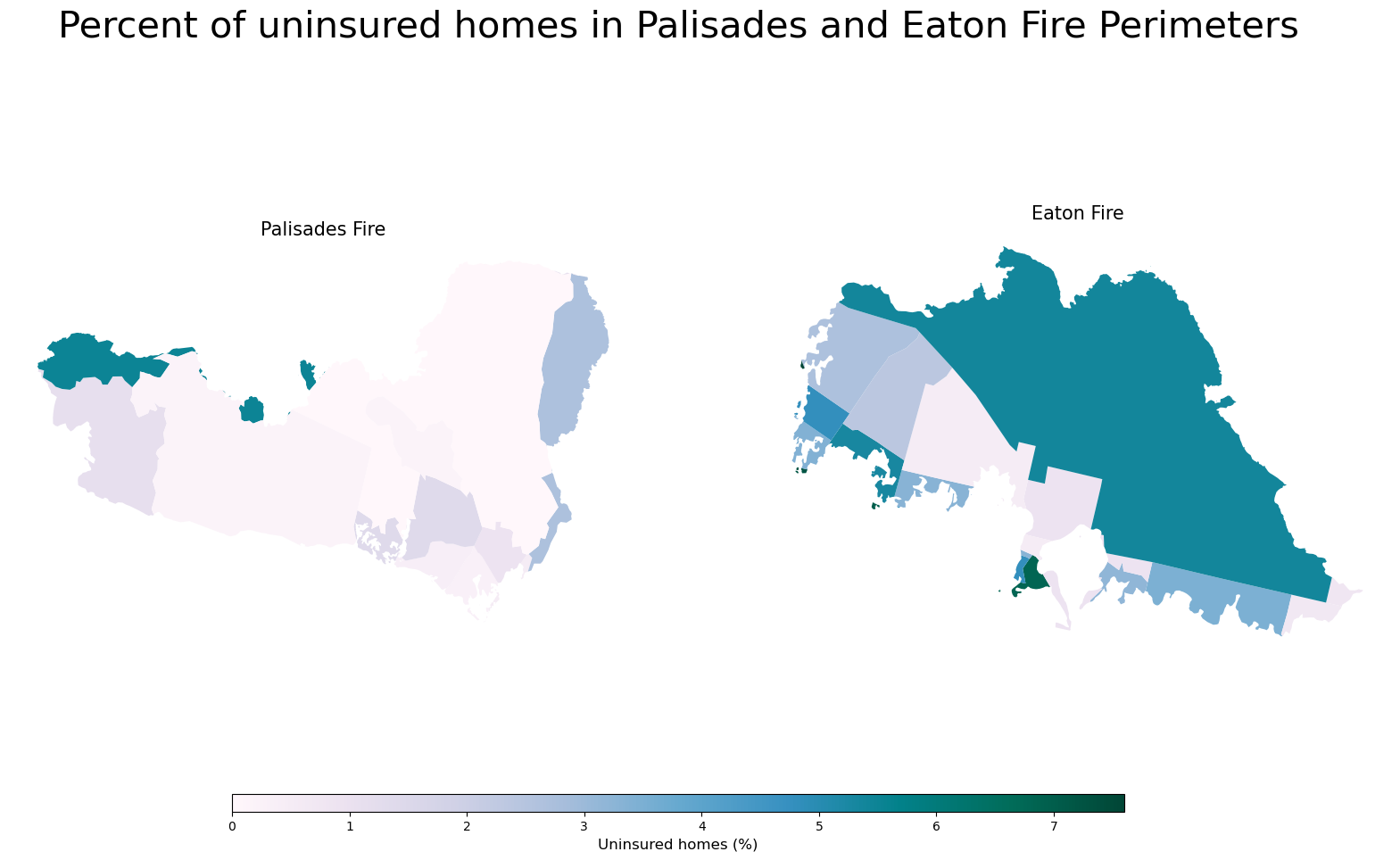

Conclusion

The Eaton and Palisades fires swept across many communities resulting in extreme damage. Through false color imagery, we visualized the burn scars in relation to the known perimeters of the fires. The percentage of uninsured homes across the Eaton fires was much greater than the percent of homes in the Palisades fires, with some areas reaching 7% of uninsured homes. This sheds light on a larger issue with insurance companies. According to an interview with NPR, many insurance companies retroactively denied coverage to many homes that experienced fires, potentially impacting more people than represented through this analysis.

References:

Overland, M. A. (2025, April 13). LA homeowners are suing insurance companies for not covering damages from the fires. NPR. https://www.npr.org/2025/04/13/nx-s1-5362537/la-homeowners-are-suing-insurance-companies-for-not-covering-damages-from-the-fires [Accessed Dec. 12, 2025]